Causal Inference with Local Polynomials

Reproduce regression-discontinuity and randomized-treatment examples with npreg, including bias-corrected inference and simultaneous grid bands.

Keywords

npreg, regression discontinuity, treatment effects, causal inference, simultaneous bands

These examples use npreg() to fit local polynomials inside two causal estimators. Each standalone script first computes a reference result with the authors’ package, then reproduces the estimate and inference using npreg plus explicit bias-correction and covariance calculations. The causal interpretation comes from the study design and its identifying assumptions.

Download a script and run it with source() in R or RStudio. It reads the pinned public data into memory, prints the numerical results, and displays the figure in your graphics window. Results remain available as rd_results or cholesterol_results; the scripts create no folders or output files. They require np 0.80-1 or later and either rdrobust or nprobust; they do not install packages. The results below were checked with np 0.80-1, rdrobust 4.1.1, and nprobust 1.0.0.

Sharp regression discontinuity

The Senate-election example estimates the discontinuity in subsequent Democratic vote share at a previous victory margin of zero. Separate fits on either side prevent smoothing across the treatment-assignment threshold. Under the RD continuity assumptions, their difference estimates a local effect of winning a close election. The data and illustration come from Calonico, Cattaneo and Titiunik (2015).

Download the complete RD script.

The script uses local linear fits, a quadratic bias-correction pilot, Epanechnikov kernels, the authors’ MSE-RD bandwidth selector, and HC0 variance estimation. Both packages use these same choices. np‘s Epanechnikov bandwidth is the authors’ bandwidth divided by $\sqrt{5}$ because the kernel support conventions differ.

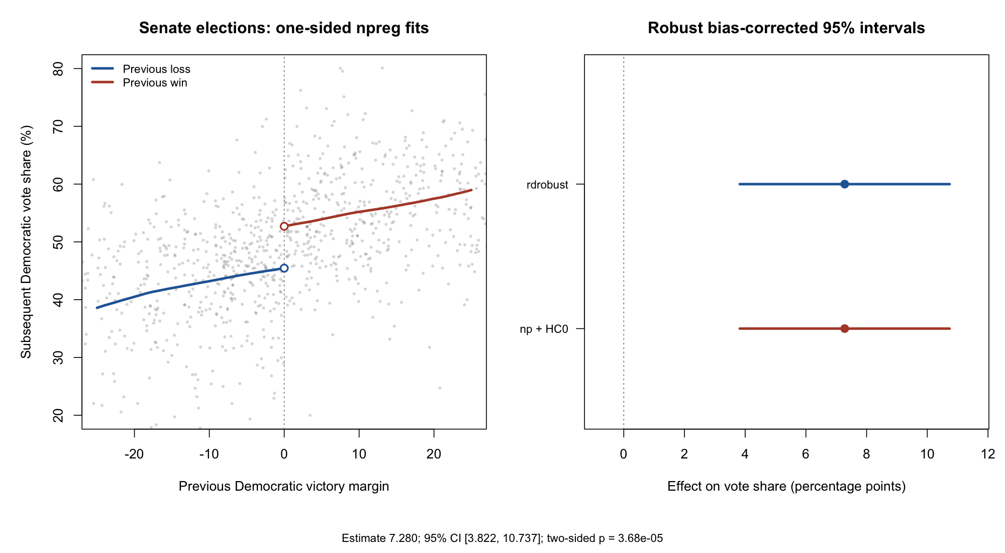
Two panels show the Senate-election discontinuity and identical robust bias-corrected confidence intervals from rdrobust and the npreg-based implementation. — Figure 1: One-sided npreg curves and matching robust bias-corrected effect intervals. The left panel shows conventional local-linear curves; the right panel shows the bias-corrected treatment-effect estimates with 95% intervals.

The conventional estimate is 7.240 percentage points; the bias-corrected estimate is 7.280, with a robust 95% interval of [3.822, 10.737]. The robust two-sided test of a zero discontinuity has $p\approx3.68\times10^{-5}$. The estimates, standard errors, interval endpoints and p-value agree to numerical precision; the script checks this directly and prints the comparison. It is also available as rd_results$comparison and as a downloadable table.

The inference follows Calonico, Cattaneo and Titiunik (2014). Epanechnikov and HC0 are supported options rather than rdrobust’s triangular kernel and nearest-neighbor variance defaults. The specialized bandwidths still come from rdrobust; ordinary regression cross-validation targets a different loss.

Complete RD code

# Sharp regression discontinuity: author package, then npreg.
# Requires np >= 0.80-1 and rdrobust. No package installation is performed.
# Run source("sharp_rd_inference.R") in R or RStudio to display the results.
# Results stay in rd_results; this script creates no folders or output files.
# References: CCT (2014), Econometrica; CCT (2015), R Journal.
# https://journal.r-project.org/articles/RJ-2015-004/
# Matched specification: Epanechnikov, p=1, q=2, MSE-RD bandwidth, HC0.
# HC0 and Epanechnikov are supported choices, not rdrobust's NN/triangular defaults.
library(np)
library(rdrobust)
stopifnot(packageVersion("np") >= "0.80.1")
options(np.messages = FALSE)
d <- read.csv(paste0(
  "https://raw.githubusercontent.com/rdpackages/rdrobust/",
  "7df239395c4afce2a58e22ef16a5817341683955/R/rdrobust_senate.csv"))
d <- d[complete.cases(d[c("vote", "margin")]), ]

# A. Author-package estimates and robust bias-corrected inference.
author <- rdrobust(y = d$vote, x = d$margin, c = 0, p = 1, q = 2,
                  kernel = "epanechnikov", bwselect = "mserd", vce = "hc0")
print(summary(author))
h <- author$bws["h", ]
b <- author$bws["b", ]
bandwidths <- data.frame(side = c("left", "right"), h, b)
print(bandwidths, row.names = FALSE)

# B. npreg fits and an explicit implementation of the same bias/HC0 formulas.
# The helper is included here so this script has no local-file dependencies.
# Local-linear robust bias correction, with a quadratic pilot and HC0 variance.
# The point estimate and second derivative are fitted by the public np API.
# Explicit equivalent weights implement the CCT/CCF covariance formula;
# np's ordinary se() uses a different residual convention.
np_rbc_hc0 <- function(x, y, at, h, b) {
  stopifnot(length(x) == length(y), all(is.finite(c(x, y, at, h, b))),
            length(at) == 1L, h > 0, b > 0)
  z <- x - at
  fit <- np::npreg(txdat = z, tydat = y, exdat = 0, bws = h / sqrt(5),
    regtype = "ll", ckertype = "epanechnikov", ckerorder = 2,
    bwtype = "fixed", bwscaling = FALSE, se = FALSE)
  pilot <- np::npreg(txdat = z, tydat = y, exdat = 0, bws = b / sqrt(5),
    regtype = "lp", degree = 2, bernstein.basis = FALSE,
    gradients = TRUE, gradient.order = 2, ckertype = "epanechnikov",
    ckerorder = 2, bwtype = "fixed", bwscaling = FALSE, se = FALSE)
  # Centered/scaled designs keep the small coefficient calculations well conditioned.
  R <- cbind(1, z / h)
  Q <- cbind(1, z / b, (z / b)^2)
  wh <- pmax(1 - (z / h)^2, 0)
  wb <- pmax(1 - (z / b)^2, 0)
  P <- solve(crossprod(R, R * wh), t(R * wh))
  B <- solve(crossprod(Q, Q * wb), t(Q * wb))
  ell <- P[1, ]
  moment2 <- sum(ell * z^2)
  ell_bc <- ell - moment2 * B[3, ] / b^2
  residual_p <- y - as.numeric(R %*% (P %*% y))
  residual_q <- y - as.numeric(Q %*% (B %*% y))
  conventional <- as.numeric(fitted(fit))
  corrected <- conventional - moment2 * as.numeric(np::gradients(pilot)) / 2
  stopifnot(abs(conventional - sum(ell * y)) < 1e-7,
            abs(corrected - sum(ell_bc * y)) < 1e-7)
  list(estimate = conventional, corrected = corrected,
       se = sqrt(sum((ell * residual_p)^2)),
       se_rb = sqrt(sum((ell_bc * residual_q)^2)),
       influence = ell_bc * residual_q)
}


sides <- list(d$margin < 0, d$margin >= 0)
fits <- lapply(1:2, function(s) {
  use <- sides[[s]]
  np_rbc_hc0(d$margin[use], d$vote[use], at = 0, h = h[s], b = b[s])
})
estimate <- fits[[2]]$estimate - fits[[1]]$estimate
corrected <- fits[[2]]$corrected - fits[[1]]$corrected
se_conventional <- sqrt(sum(vapply(fits, function(f) f$se^2, 0)))
se_robust <- sqrt(sum(vapply(fits, function(f) f$se_rb^2, 0)))
ci <- corrected + c(-1, 1) * qnorm(.975) * se_robust
p_value <- 2 * pnorm(-abs(corrected / se_robust))
comparison <- data.frame(
  quantity = c("Conventional estimate", "Bias-corrected estimate", "Conventional SE",
               "Robust SE", "Robust CI lower", "Robust CI upper", "Robust p-value"),
  author = c(author$Estimate[1, ], author$ci["Robust", ], author$pv["Robust", 1]),
  np = c(estimate, corrected, se_conventional, se_robust, ci, p_value))
comparison$absolute_difference <- abs(comparison$author - comparison$np)
stopifnot(max(comparison$absolute_difference) < 1e-7)
print(comparison, digits = 8, row.names = FALSE)
rd_results <- list(data = d, author = author, bandwidths = bandwidths,
                   comparison = comparison, session_info = sessionInfo())

# Display conventional np curves and the two identical RBC effect intervals.
gx <- list(seq(-25, 0, length.out = 151), seq(0, 25, length.out = 151))
gy <- lapply(1:2, function(s) as.numeric(fitted(npreg(
  txdat = d$margin[sides[[s]]], tydat = d$vote[sides[[s]]], exdat = gx[[s]],
  bws = h[s] / sqrt(5), regtype = "ll", ckertype = "epanechnikov",
  ckerorder = 2, bwtype = "fixed", bwscaling = FALSE, se = FALSE))))
if (interactive() || dev.cur() > 1L) local({
  old_par <- par(no.readonly = TRUE)
  on.exit(par(old_par))
  par(mfrow = c(1, 2), mar = c(5.7, 5.1, 3.4, 1.0), oma = c(2.0, 0, 0, 0))
  cols <- c("#2667A5", "#B24A35")
  plot(d$margin, d$vote, xlim = c(-25, 25), ylim = c(20, 80),
       pch = 16, cex = .5, col = adjustcolor("grey40", .25),
       xlab = "Previous Democratic victory margin", ylab = "Subsequent Democratic vote share (%)",
       main = "Senate elections: one-sided npreg fits")
  abline(v = 0, lty = 3, col = "grey50")
  for (s in 1:2) {
    lines(gx[[s]], gy[[s]], lwd = 3, col = cols[s])
    points(0, fits[[s]]$estimate, pch = 21, bg = "white", col = cols[s], cex = 1.2, lwd = 2)
  }
  legend("topleft", c("Previous loss", "Previous win"), col = cols, lty = 1, lwd = 3, bty = "n", cex = .85)
  plot(NA, xlim = range(0, ci) + c(-.8, .8), ylim = c(.4, 2.8), yaxt = "n",
       xlab = "Effect on vote share (percentage points)", ylab = "",
       main = "Robust bias-corrected 95% intervals")
  abline(v = 0, col = "grey50", lty = 3)
  axis(2, at = c(1, 2), labels = c("np + HC0", "rdrobust"), las = 1, cex.axis = .85)
  segments(author$ci["Robust", 1], 2, author$ci["Robust", 2], 2, lwd = 3, col = cols[1])
  segments(ci[1], 1, ci[2], 1, lwd = 3, col = cols[2])
  points(c(author$Estimate[1, "tau.bc"], corrected), c(2, 1), pch = 19, col = cols, cex = 1.3)
  mtext(sprintf("Estimate %.3f; 95%% CI [%.3f, %.3f]; two-sided p = %.3g", corrected, ci[1], ci[2], p_value),
        side = 1, outer = TRUE, line = .5, cex = .85)
}) else message('Run source("sharp_rd_inference.R") in R or RStudio to display the figure.')
invisible(rd_results)

Randomized treatment effects with simultaneous bands

The cholesterol example uses the Efron–Feldman randomized-trial data supplied with nprobust. It compares expected post-treatment cholesterol between assignment groups, conditional on pre-treatment cholesterol. There are 172 control and 165 treatment observations. The post-treatment compliance variable is not used. The regression illustration follows Calonico, Cattaneo and Farrell (2019).

Download the complete cholesterol script.

Each arm uses local linear regression with the authors’ IMSE-DPI bandwidths, a quadratic bias correction, Epanechnikov kernels and HC0 covariance. The effect is the difference between the two bias-corrected means; the covariance matrices add across the independent arms. npreg supplies the regression and second-derivative pilot fits, and the script reproduces the authors’ full covariance across evaluation points.

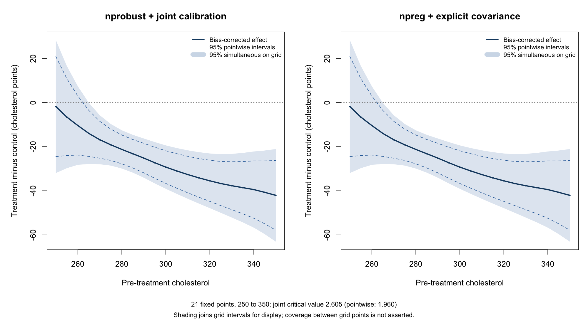
Two matching panels compare nprobust-based and npreg-based bias-corrected cholesterol treatment effects. Blue shading is the 95 percent simultaneous grid band and dashed lines show narrower pointwise intervals. — Figure 2: Matching treatment-effect curves, pointwise intervals and simultaneous grid bands. Shading represents approximate 95% simultaneous coverage over the 21 specified baseline-cholesterol values.

The simultaneous band is an additional inference step, applied identically to both implementations. It uses 50,000 joint Gaussian draws, seed 20261011, and the maximum absolute standardized deviation across the fixed grid $250,255,\ldots,350$. The resulting critical value is 2.605, versus 1.960 for pointwise intervals. This calibration preserves dependence between the estimates; the general Gaussian-maximum approach is discussed by Chernozhukov, Chetverikov and Kato (2013).

The same calibration tests whether the effect is zero at every grid point. Here the maximum statistic is 7.779, exceeding every simulated maximum. The reported Monte Carlo p-value is at its resolution limit, about $2\times10^{-5}$; it is not an exact tail probability. This rejects the all-zero curve, while the band still includes zero at baseline values 250, 255 and 260. It does not establish an effect everywhere or test whether the effect is constant.

Coverage is approximate and simultaneous over these 21 points, not every point of a continuous interval. The shaded polygon joins intervals for display. The calculation holds the selected bandwidths fixed and relies on the usual asymptotic conditions, including sufficiently small remaining bias after correction. These are confidence bands for the conditional mean contrast, not prediction bands for individual outcomes.

The script checks the bias-corrected estimates, standard errors, covariance, band endpoints and joint test against the author-package calculation. Inspect cholesterol_results$np_band and cholesterol_results$joint_test in R, or download the np band values, author-package band values, numerical checks, or joint-test results.

Complete cholesterol code

# Conditional treatment effects: author package, then npreg, with simultaneous bands.
# Requires np >= 0.80-1 and nprobust (tested with 1.0.0). No installation is performed.
# Run source("cholesterol_simultaneous.R") in R or RStudio to display the results.
# Results stay in cholesterol_results; no folders or output files are created.
# Calonico, Cattaneo & Farrell (2019), https://doi.org/10.18637/jss.v091.i08
# Trial data: Efron & Feldman (1991). t is randomized assignment, not compliance.
# Author-supported choices: Epanechnikov, p=1, IMSE-DPI, HC0 (rather than default NN).
# The joint Gaussian calibration is an added finite-grid inference step, not an
# nprobust default or a replication of a simultaneous band printed in the article.
library(np)
library(nprobust)
stopifnot(packageVersion("np") >= "0.80.1")
options(np.messages = FALSE)
d <- read.csv(paste0(
  "https://raw.githubusercontent.com/nppackages/nprobust/",
  "dfcb562d34822c75528c1c2d8a5a153be6b3a683/R/nprobust_data.csv"))
stopifnot(all(complete.cases(d[c("t", "chol1", "cholf")])) , all(d$t %in% 0:1))
grid <- seq(250, 350, by = 5) # Fixed 21-point target; no continuum-coverage claim.

# A. Author-package fits and their full robust covariance across the grid.
author <- lapply(0:1, function(arm) {
  use <- d$t == arm
  lprobust(y = d$cholf[use], x = d$chol1[use], eval = grid,
           p = 1, kernel = "epa", bwselect = "imse-dpi", vce = "hc0", covgrid = TRUE)
})
author_tau <- author[[2]]$Estimate[, "tau.bc"] - author[[1]]$Estimate[, "tau.bc"]
author_V <- author[[1]]$cov.rb + author[[2]]$cov.rb # independent randomized arms
bandwidths <- do.call(rbind, lapply(0:1, function(arm) data.frame(arm,
  x = grid, h = author[[arm + 1]]$Estimate[, "h"], b = author[[arm + 1]]$Estimate[, "b"])))

# B. Public npreg calls for point and pilot fits; explicit CCF HC0 covariance.
# Helpers are included so this script has no local-file dependencies.
# Local-linear robust bias correction, with a quadratic pilot and HC0 variance.
# The point estimate and second derivative are fitted by the public np API.
# Explicit equivalent weights implement the CCT/CCF covariance formula;
# np's ordinary se() uses a different residual convention.
np_rbc_hc0 <- function(x, y, at, h, b) {
  stopifnot(length(x) == length(y), all(is.finite(c(x, y, at, h, b))),
            length(at) == 1L, h > 0, b > 0)
  z <- x - at
  fit <- np::npreg(txdat = z, tydat = y, exdat = 0, bws = h / sqrt(5),
    regtype = "ll", ckertype = "epanechnikov", ckerorder = 2,
    bwtype = "fixed", bwscaling = FALSE, se = FALSE)
  pilot <- np::npreg(txdat = z, tydat = y, exdat = 0, bws = b / sqrt(5),
    regtype = "lp", degree = 2, bernstein.basis = FALSE,
    gradients = TRUE, gradient.order = 2, ckertype = "epanechnikov",
    ckerorder = 2, bwtype = "fixed", bwscaling = FALSE, se = FALSE)
  # Centered/scaled designs keep the small coefficient calculations well conditioned.
  R <- cbind(1, z / h)
  Q <- cbind(1, z / b, (z / b)^2)
  wh <- pmax(1 - (z / h)^2, 0)
  wb <- pmax(1 - (z / b)^2, 0)
  P <- solve(crossprod(R, R * wh), t(R * wh))
  B <- solve(crossprod(Q, Q * wb), t(Q * wb))
  ell <- P[1, ]
  moment2 <- sum(ell * z^2)
  ell_bc <- ell - moment2 * B[3, ] / b^2
  residual_p <- y - as.numeric(R %*% (P %*% y))
  residual_q <- y - as.numeric(Q %*% (B %*% y))
  conventional <- as.numeric(fitted(fit))
  corrected <- conventional - moment2 * as.numeric(np::gradients(pilot)) / 2
  stopifnot(abs(conventional - sum(ell * y)) < 1e-7,
            abs(corrected - sum(ell_bc * y)) < 1e-7)
  list(estimate = conventional, corrected = corrected,
       se = sqrt(sum((ell * residual_p)^2)),
       se_rb = sqrt(sum((ell_bc * residual_q)^2)),
       influence = ell_bc * residual_q)
}

# Conditional Gaussian calibration, simultaneous over a FIXED finite grid.
# The same draw is shared across all points through the joint covariance.
grid_max_t <- function(covariance, estimate, B = 50000L, seed = 20261011L) {
  se <- sqrt(diag(covariance))
  stopifnot(all(is.finite(se)), all(se > 0))
  correlation <- covariance / outer(se, se)
  root <- chol(correlation) # Fail if the supplied covariance is not positive definite.
  set.seed(seed)
  draws <- matrix(rnorm(nrow(root) * B), nrow(root), B)
  maxima <- apply(abs(t(root) %*% draws), 2, max)
  statistic <- max(abs(estimate / se))
  list(critical = unname(quantile(maxima, 0.95, type = 1)),
       statistic = statistic, p = (1 + sum(maxima >= statistic)) / (B + 1),
       B = B, seed = seed, se = se)
}

np_fits <- np_cov <- list()
checks <- list()
for (arm in 0:1) {
  use <- d$t == arm
  ref <- author[[arm + 1]]$Estimate
  fits <- lapply(seq_along(grid), function(j) np_rbc_hc0(
    d$chol1[use], d$cholf[use], grid[j], h = ref[j, "h"], b = ref[j, "b"]))
  np_fits[[arm + 1]] <- t(vapply(fits, function(z) c(z$estimate, z$corrected, z$se, z$se_rb), numeric(4)))
  colnames(np_fits[[arm + 1]]) <- c("tau.us", "tau.bc", "se.us", "se.rb")
  np_cov[[arm + 1]] <- tcrossprod(do.call(rbind, lapply(fits, `[[`, "influence")))
  checks[[arm + 1]] <- data.frame(arm,
    max_estimate_se_error = max(abs(np_fits[[arm + 1]] - ref[, colnames(np_fits[[arm + 1]])])),
    max_covariance_error = max(abs(np_cov[[arm + 1]] - author[[arm + 1]]$cov.rb)))
}
checks <- do.call(rbind, checks)
stopifnot(max(as.matrix(checks[-1])) < 1e-7)
np_tau <- np_fits[[2]][, "tau.bc"] - np_fits[[1]][, "tau.bc"]
np_V <- np_cov[[1]] + np_cov[[2]]

# C. Same joint calibration applied independently to both implementations.
# Bandwidths are held fixed. Standard asymptotic conditions, including negligible
# remaining bias after correction, are needed. These are approximate 95% bands.
author_cal <- grid_max_t(author_V, author_tau)
np_cal <- grid_max_t(np_V, np_tau)
stopifnot(abs(author_cal$critical - np_cal$critical) < 1e-7,
          abs(author_cal$statistic - np_cal$statistic) < 1e-7,
          author_cal$p == np_cal$p)
band <- function(tau, cal) data.frame(x = grid, estimate = tau, se = cal$se,
  point_lower = tau - qnorm(.975) * cal$se, point_upper = tau + qnorm(.975) * cal$se,
  simultaneous_lower = tau - cal$critical * cal$se,
  simultaneous_upper = tau + cal$critical * cal$se)
author_band <- band(author_tau, author_cal)
np_band <- band(np_tau, np_cal)
stopifnot(max(abs(as.matrix(author_band - np_band))) < 1e-7)
test <- data.frame(method = c("nprobust + joint calibration", "npreg + explicit covariance"),
  critical = c(author_cal$critical, np_cal$critical),
  max_t = c(author_cal$statistic, np_cal$statistic),
  monte_carlo_p = c(author_cal$p, np_cal$p), B = np_cal$B, seed = np_cal$seed)
print(checks, digits = 6)
print(test, digits = 6, row.names = FALSE)
cat("Test null: treatment effect equals zero at every one of the 21 grid points.\n",
    "This does not test whether the treatment effect is constant.\n",
    "The Monte Carlo p-value has resolution 1/(B+1); a floor value is not an exact tail probability.\n")
cholesterol_results <- list(data = d, author = author, bandwidths = bandwidths,
  author_band = author_band, np_band = np_band, checks = checks, joint_test = test,
  session_info = sessionInfo())

if (interactive() || dev.cur() > 1L) local({
  old_par <- par(no.readonly = TRUE)
  on.exit(par(old_par))
  par(mfrow = c(1, 2), mar = c(5.1, 5.0, 3.4, 1.0), oma = c(2.7, 0, 0, 0))
  limits <- range(author_band[c("simultaneous_lower", "simultaneous_upper")], 0)
  for (s in 1:2) {
    tab <- list(author_band, np_band)[[s]]
    plot(grid, tab$estimate, type = "n", ylim = limits,
         xlab = "Pre-treatment cholesterol", ylab = "Treatment minus control (cholesterol points)",
         main = c("nprobust + joint calibration", "npreg + explicit covariance")[s])
    polygon(c(grid, rev(grid)), c(tab$simultaneous_lower, rev(tab$simultaneous_upper)),
            col = adjustcolor("#2667A5", .16), border = NA)
    abline(h = 0, col = "grey50", lty = 3)
    lines(grid, tab$point_lower, col = "#2667A5", lty = 2)
    lines(grid, tab$point_upper, col = "#2667A5", lty = 2)
    lines(grid, tab$estimate, col = "#174970", lwd = 2.5)
    points(grid, tab$estimate, col = "#174970", pch = 16, cex = .45)
    legend("topright", c("Bias-corrected effect", "95% pointwise intervals", "95% simultaneous on grid"),
           col = c("#174970", "#2667A5", adjustcolor("#2667A5", .25)),
           lty = c(1, 2, 1), lwd = c(2.5, 1, 9), bty = "n", cex = .8)
  }
  mtext(sprintf("21 fixed points, 250 to 350; joint critical value %.3f (pointwise: 1.960)", np_cal$critical),
        side = 1, outer = TRUE, line = .15, cex = .85)
  mtext("Shading joins grid intervals for display; coverage between grid points is not asserted.",
        side = 1, outer = TRUE, line = 1.25, cex = .82)
}) else message('Run source("cholesterol_simultaneous.R") in R or RStudio to display the figure.')
invisible(cholesterol_results)

Observational treatment effects with cross-fitting

For a workflow with many adjustment covariates, see Doubly Robust Treatment Effects. That companion example follows Fan, Hsu, Lieli and Zhang: estimate nuisance functions outside each held-out fold, construct doubly robust scores, and use npreg for the final local-linear CATE curves. A seeded simulation with known truth shows pointwise intervals and simultaneous multiplier bands. The page explains the identifying assumptions and the explicit exponential-weight choice, and supplies a standalone script and reference-verification notes.

Difference-in-differences with changing composition

For repeated cross-sectional data, see Difference-in-Differences with Changing Composition. That example revisits Sant’Anna and Xu’s tariff-evasion application, freshly estimating generalized propensities with npconmode and outcome regressions with npreg. A standalone script produces the published/np ATT comparison table and clustered standard errors. The page explains the adaptations and their broad agreement with the published results.

What is supplied by np?

In the RD and trial examples above, npreg supplies the local-polynomial point and pilot fits. The scripts add the cited bias correction and HC0 covariance formulas explicitly: ordinary se() and plotting bands use different uncertainty conventions and are not substitutes for these calculations. The authors’ packages supply the specialized bandwidths and serve as numerical references. The simultaneous contrast band is an extension of their pointwise example, not a band claimed to appear in the original article.

For other fitting and plotting examples, see Worked Examples and Plotting and Intervals.